Dynamic Positioning of Totals using Dynamic Arrays
In the video above you learned how to create Dynamic Positioning of Totals using Dynamic arrays using Excels SEQUENCE function and some logic. This is an awesome trick that will give any spreadsheet that look professional.
As promised in the video, I have a Learn and Earn Activity for you to complete so you can practice what you have learned.
Download the file. It contains the sample data as shown in the image.
https://www.dropbox.com/s/l8fza7gnb214av1/dynamictotals.xlsx?dl=0
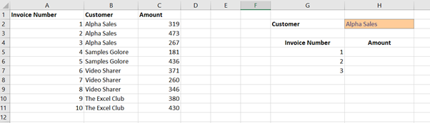
Column A:C contains the data we wish to work with. Cell H2 contains data validation allowing you to select between the customer.
The aim of the task is to pull in the Amount of the invoice into column H, and to include a total value of all invoices.
To aid with this, I have already included a dynamic array formula to pull in the invoice numbers for the selected customer.
Dynamic positioning of totals Learn and Earn Activity
In the comments section below detail the steps and the formula you used to pull in the amount for the invoices and a Dynamic total.
The way shown in the video is not the only way to do this. There are alternatives. If you have an alternative please do share it as you may be providing a valuable resource for someone else.
Do you want to start collecting rewards quickly for learning Excel? Then you should try:
10+ Excel Learn and Earn Activities YOU can do Today
SIGN UP FOR OUR NEWSLETTER TODAY – GET EXCEL TIPS TRICKS AND LEARN AND EARN ACTIVITIES TO YOUR INBOX
SIGN UP
Congratulations @theexcelclub! You have completed the following achievement on the Steem blockchain and have been rewarded with new badge(s) :
You can view your badges on your Steem Board and compare to others on the Steem Ranking
If you no longer want to receive notifications, reply to this comment with the word
STOPTo support your work, I also upvoted your post!
Vote for @Steemitboard as a witness to get one more award and increased upvotes!
Hello,
Your post has been manually curated by a @stem.curate curator, @balticadger.
We are dedicated to supporting great content, like yours on the STEMGeeks tribe.
If you like what we are doing, please show your support as well by following our Steem Auto curation trail.
Please join us on discord.
There is conditional format for Total (i.e, Bold and Lines). How it is done?.
- Kishore Kumar
you can find out how to do that in this post
https://theexcelclub.com/excel-dynamic-conditional-formatting-tricks/
@paulag Paula, is the video above on how to create Dynamic Positioning of Totals using Dynamic arrays using Excels SEQUENCE function, has anything to do with the above Learn and Earn Activity? Are the both using the same method? I'm sorry I kind of confuse right now.
the learn and earn activity on this post is
"In the comments section below detail the steps and the formula you used to pull in the amount for the invoices and a Dynamic total.
The way shown in the video is not the only way to do this. There are alternatives. If you have an alternative please do share it as you may be providing a valuable resource for someone else."
I got it. Thank you, Paula.
For pull in the Amount of the invoice into column H:
In cell H5, I typed in =SUMIFS(C1:C11,A1:A11,A2).
In cell H6, I typed in =SUMIFS(C1:C11,A1:A11,A3).
In cell H7, I typed in =SUMIFS(C1:C11,A1:A11,A4).
For total value of all invoices:
In cell H8, I typed in =SUM(H5:H7). That gives a total of 1059.
Paula, am I doing it right? I hope that I'm doing it right.
without dynamic arrays, you would enter a formula to each cell. Have you tried it with dynamic arrays? ( what version of Excel are you using?)
I have went through the video above and I couldn't get the understanding on how to apply the dynamic arrays onto the Learn and Earn Activity above without entering a formula to each cell.
I'm using my laptop that installed with "Linux Mint 19.1 Cinnamon" OS.
I'm using FreeOffice PlanMaker 2018 (rev 973.1103) 64bit.
It is an alternate version of Excel for my Linux OS laptop.
ah, so you don't have the dynamic arrays feature in the package you are using. you could try excel online :-)
Okay, I will use Excel online.
This is what I did using Microsoft Excel online.
For pull in the Amount of the invoice into column H:
In cell H5, as I typed in =SUM, a drop-down list appeared, and I double-click on SUMIFS and =SUMIFS( filled in the cell H5. Then, I clicked and dragged from cell C1 to cell C11. Then, I typed ',' and then I clicked and dragged from cell A1 to cell A11. Then, I typed ',' and then I clicked on cell A2, and then I typed ')' and press Enter. Number 319 filled in the cell H5.
In cell H6, as I typed in =SUM, a drop-down list appeared, and I double-click on SUMIFS and =SUMIFS( filled in the cell H6. Then, I clicked and dragged from cell C1 to cell C11. Then, I typed ',' and then I clicked and dragged from cell A1 to cell A11. Then, I typed ',' and then I clicked on cell A3, and then I typed ')' and press Enter. Number 473 filled in the cell H6.
In cell H7, as I typed in =SUM, a drop-down list appeared, and I double-click on SUMIFS and =SUMIFS( filled in the cell H7. Then, I clicked and dragged from cell C1 to cell C11. Then, I typed ',' and then I clicked and dragged from cell A1 to cell A11. Then, I typed ',' and then I clicked on cell A4, and then I typed ')' and press Enter. Number 267 filled in the cell H7.
For total value of all invoices:
In cell H8, as I typed in =SUM, a drop-down list appeared, and I double-click on SUM and =SUM( filled in the cell H8. Then, I clicked and dragged from cell H5 to cell H7. Then, I typed ')' and press Enter. Number 1059 filled in the cell H8.