Excel Dynamic Arrays – A new way to model your Excel Spreadsheets
Excel Dynamic Arrays – changing how Excel works
Many years ago, I heard Excel referred to as ‘Hell in a Cell’. I don’t know who coined this statement, but I have used it many times myself. In one cell you can only have 1 value. For every value, you need to enter either that value, or a formula to return a value. And each formula will return only one value. And that’s the way Excel works. Or that’s the way Excel did work.
Dynamic Arrays and Spill areas. Excel is moving from hell in a cell, to a whole new way of calculating. The entire calculation grid is changing how it works. It is becoming more powerful, faster and less prone to error. Now you will be able to create one formula and return many values.
Along with Dynamic Arrays and Spill areas are 6 new functions. FILTER, RANDARRAY, SQEUENCE, SORT, SORTBY and UNIQUE. But dynamic arrays are not limited to these new functions.
The possibilities are now endless. The way we work in Excel is about to change dramatically. Traditional Array functions entered using Ctrl + Shift + Enter to get those curly brackets are no longer for advanced users. CTRL + Shift + Enter is gone, along with the brackets. Excel will think in arrays and expect to return multiple values instead of one.
Dynamic Arrays Example 1 – Creating a Unique List
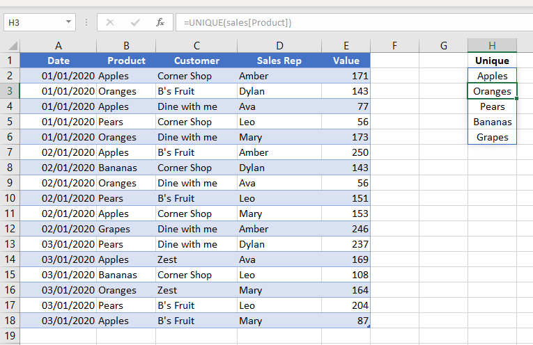
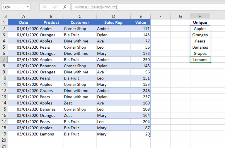
Consider the following table of sales data, although small, it is perfect for our example.
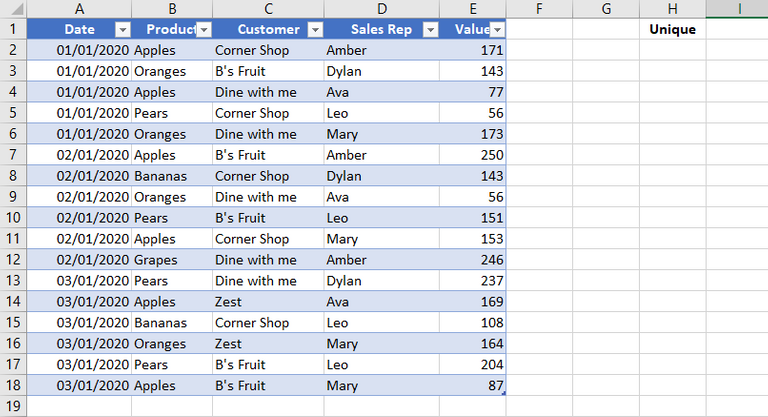
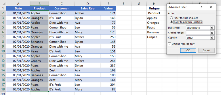
Suppose you need a unique list of Products. Under the old Excel it was a bit of a headache. You can do this this a number of ways depended on your needs and knowledge. You could write a complex formula. Or, you could load the data into Power Query, or you could use Advanced Filter.
Advanced Filter is okay if you are working with static data. If your column changes, you would have to re-run advanced filter to get a new unique list. I have often seen this method used by less experienced excel users. Then they wonder why things like data validation break!
There are just too many steps when using Power Query for the sole purpose of extracting a unique list. And if you were to use a formula, it would be a complex array formula. Way beyond the ability of most Excel users.
However, with Excels new array thinking and the new UNIQUE function, obtaining unique list is simple.
UNIQUE Function in Excel
The syntax for UNIQUE is
=UNIQUE(array, [by_col], [occurs_once])
We will explore the full detail of the UNIQUE function at a later stage. But as we know parameters in excel functions surrounded with square brackets [ ] can often be left out as they are optional.
Therefore, to get a unique list of the Products, the only parameter we need to feed the UNIQUE function is the array.
By using the formula =UNIQUE(sales[Products]) in only one cell, we can get a unique list.
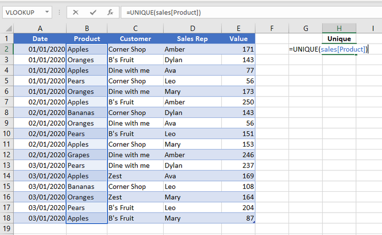
As we entered an array, Excel knows to return an array, or more than one value. On hitting Enter, not only will the cell with the formula return a value, but the unique list will Spill down to other cells.
Recognizing and Working with Excel Dynamic Arrays
You will note from our UNIQUE example, 5 items were returned and these filled the column down. We did not enter formulas into the other cells. The range in which the function fills is known as the Spill range. By selecting any of the cells in the Spill range, a blue box will appear allowing you identify the entire spill range.
You will see the formulas in grey throughout the Spill range. You can not edit the formula in any of the Spill cells. It can only be edited in the cell in which it was entered.
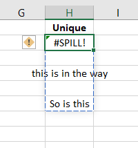
If you have values in the Spill Range, you will get a Spill error. By selecting the cell with the error, a blue dotted line will show you where the Spill range wants to fill.
By clicking on the Formula warning, you can quickly select all obstruction cells, and delete, or move the data somewhere else.
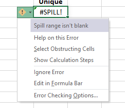
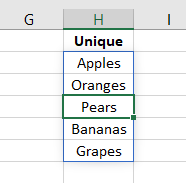
Once you have cleared the area Excel wants to fill to, the error will be fixed and the results will spill.
This spill range is also dynamic. In our example we have the source data stored in table format. Hence the formula UNIQUE(sales[Products]) and not UNIQUE(B2:B18). If we now update this table with a new row of data, and a new product, the UNIQUE function also updates, and the Spill range expands.
Are you starting to see the benefits of the new calculation engine in Excel? By entering a formula only once, you are saving a lot of time, and you are less prone to error. More efficient and accurate. How cool is that. But wait, there is more, loads more.
Referencing values from Spill Ranges
You can use values from a Spill Range as an input to other formulas or features.
To reference ALL the values contained within a dynamic array, reference only the cell with the formula and then add # to the end. You can also reference the values from each cell within the spill range, by selecting just that cell.
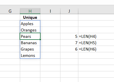
For Example, we can use the function LEN to get the number of characters in each word. In this example = LEN(H4) we have referenced the actual cells reference H4. We can see the number of characters returned is correct at 5. The driving cell, H4, does not ‘really’ contain any values, as it is part of a spill range. If we copy this formula down, it works just like any Excel formula referencing a value from within a cell.
You can reference the entire Spill Range by adding the symbol # to the end of the cell reference that contains the dynamic array formula. For example, as per the image, in cell J2 is =LEN(H2#). Once we add the # the Dynamic array spill will be selected. The result is a spill showing the LEN of each value in our unique list.
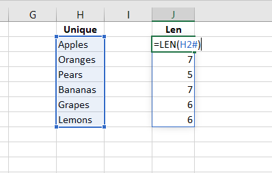
The Spill in this case is 6 values. In old Excel, we would need 6 formulas entered into Excel to return these 6 values. We did not need to fill down the formula and we did not need to press CTRL+Shift+Enter for Excel to return an array.
Dynamic Arrays Example 2 – Dynamic Data Validation and SORT
With Dynamic Spill ranges, Excels Sort and Filter options do not work. Therefore, Microsoft have introduced new functions to help with this. SORT and FILTER functions.
We will look at both function in more detail at a different time. For now, we are going to take a quick look at SORT, so we can create a Sorted unique list to be use in a Data Validation drop down.
The syntax for sort is
SORT(array, [sort index], [sort order], [by col])
However we know the items in [ ] can be omitted. The default sort order in the SORT function is Ascending order. So, to sort our unique list A-Z we only need to enter the array to the function.
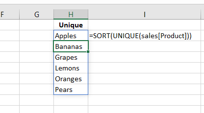
As the UNIQUE function returns an Array, we can use this array in our SORT function. =SORT(UNIQUE(sales[Product])) will therefore return a sorted unique list of our products.

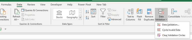
We can then use this list to create a Dynamic Data validation drop down. You will find Data validation on the Data Ribbon.
In the data validation window, select Allow List. In the Source reference only the cell that contains the formula, in this case $H2$. We then add # to the end of the cell reference to tell Excel is it the Spill array that you want.
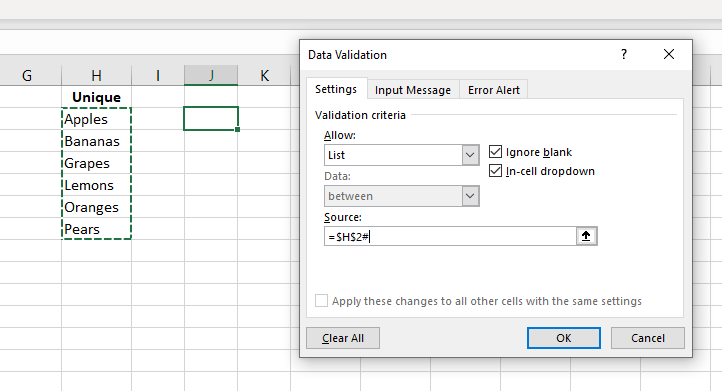
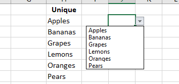
This will then create a dynamic drop down. The drop down will update as the unique list updates making it dynamic at all times.
Dynamic Arrays Example 3 – Transporting a Unique List
We have seen how a function spills down when we select a column. If we take a Row of values as our array, the spill will also go across the row. However, what if you needed values from a column to spill over a row? How would you go about this?
Well we can simply wrap our UNIQUE function between the TRANSPOSE function. The TRANSPOSE function is a old array formula that existed in Excel. Its syntax is
=TRANSPOSE(array)
We know our UNIQUE function returns an array. and if we had this UNIQUE wrapped in SORT, we would also have an array. Now we can just wrap TRANSPOSE around this.
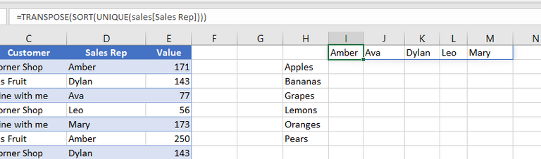
For this example we will take a unique list of the Sales Rep.
=TRANSPOSE(SORT(UNIQUE(sales[Sales Rep])))
Dynamic Arrays Example 4 – 3 Formulas, 1 pivot table.
Did you every think you could create a calculation table like a pivot table using formulas. With Dynamic arrays, this becomes very simple.
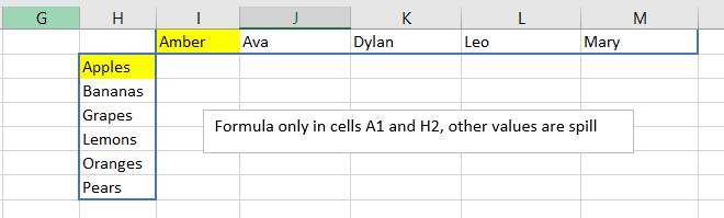
Using only 2 formulas we have been able to create a column containing unique products and a row containing unique Sales Reps.
Now with only 1 more formula, we can get the total Value for each product by each Sales rep. Something most of us would only have considered calculating using a pivot table.
In cell I2 we are going to create a SUMIFS function. If you are not familiar with SUMIFS in Excel you can read this article here .
SUMIFS will allow you sum by multiple criteria. In our table, we have both Products and Sales Rep and we want to sum the VALUE for each
The syntax for SUMIFS is
=SUMIFS(Sum Range, Criteria Range 1, Criteria 1, [Criteria range 2, Criteria 2)….).
The formula we will use is
=SUMIFS(sales[Value],sales[Product],$H$2#,sales[Sales Rep],$I$1#)
The Sum range sales[Value] is the value we want to sum
Criteria range is the range where you will find the criteria defining what you want to sum. This is case we want to sum the Sales value, first based on the Sales[Product].
Next we define the first criteria we want to sum by. H2 contains Apples. However, we don’t just want Apples, we want all of the array. So, we use the # after the cell reference $H2$#.
The SUMIFS function then moves on to the second criteria. Taking the Sales Rep column, filter to the sales rep shown in the Spill array and then sum the values.
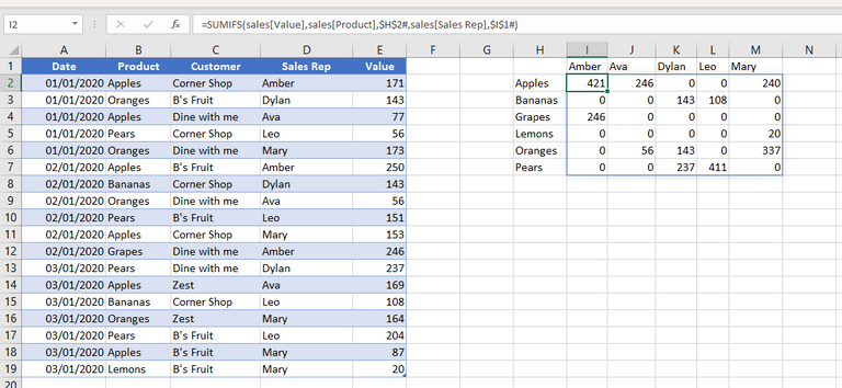
As we have taken the Spill ranges in our SUMIFS formula, the values returned for this formula will also spill.
Benefits Over Pivot tables
Creating a calculation table like this with only 3 formulas is very much a game changer. Before, if we created such a table using Excel Pivot Table features, the Pivot table would need a Refresh when source data table is updated.
However, with the user of Dynamic Arrays, there is no need to refresh as these arrays are truly dynamic and will update for you when you update your table.
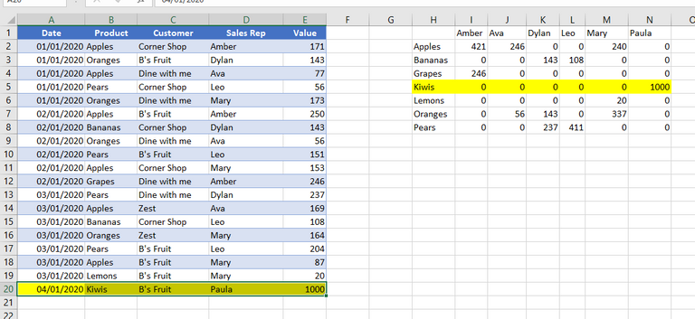
As you can see this is fast, it is reliable, and it is less prone to human error. You do not have to remember to refresh and you don’t have to update any formulas. In addition, it also took only 3 formulas to create.
Backward Compatibility
The 6 new functions that arrive with Dynamic Arrays are not backward compatible. Neither is the spill range operator. However, if you open an Excel workbook in an earlier version, the values will remain intact and you can use these values in other formulas. But once you try edit the formula, it will break. You will note these formulas as in the formula bar you will see _xlfn, which indicates the formula is not supported.
When you open a workbook containing Dynamic Arrays in an older version, Excel will convert these to its only array structure. These will include the curly brackets and if you edit these formulas remember to press CTRL+Shift+Enter.
Conclusion
This new calculation engine and Excel Dynamic Arrays are only available in Excel 365 (currently insiders edition only). I have to say these changes are really amazing and they will completely change how I go about creating spreadsheets and models moving forward.
In this article we looked at only a few small examples. And we did not take a deep dive into any of the new functions. Instead I tried to select a few examples that would first show you how Dynamic Arrays work. And the show you some of the capabilities available when you use Dynamic Arrays with existing functions such as SUMIFS.
Learn and Earn Activity
Are you excited about this change and the introduction of Excel Dynamic Arrays? Leave a comment below telling us what you think of these changes and how you can see your self apply them.
If you are already working with Dynamic Arrays in Excel, share with us how you are using them and what benefit they have give you.
Comments that add value to this post and to other readers will be rewarded. Find out more about our Worlds Exclusive Learn and Earn Excel Activities by clicking here
IF YOU CARE YOU WILL SHARE - PLEASE USE THE SHARE BUTTONS BELOW THE POST
NEWSLETTER SIGN UP - SIGN UP NOW AND NEVER MISS AN EXCEL TRICK AGAIN

- includes XLOOKUP and will soon include Dynamic Arrays


Power Query Excel 365

The Excel Club is the only Excel Blog in the world where you can Earn while you Learn Excel. Find out about our Learn and Earn Activities now
SIGN UP FOR OUR NEWSLETTER AND GET EXCEL & POWER BI TIPS TRICKS AND TUTORIAL TO YOUR INBOX
SIGN UP NOW

Cross posted from my blog with SteemPress : https://theexcelclub.com/excel-dynamic-arrays-a-new-way-to-model-your-excel-spreadsheets/
I think the changes of Excel Dynamic Arrays are beneficial because it let excel users learn more advanced features of using Microsoft excel. I can see myself applying the feature to the best of my ability when using excel in the future.
- Kenroy Hunter
This is way ahead of my level, but interesting indeed. Would this be used to replace relative and absolute cell references too? I have only started to really understand those.
Anything that would make my job easier is good. So am I excited by this new feature, yes indeed. How will I use it moving forward? I will have to watch more of your videos and articles to see how to apply dynamic arrays
wow Paula I am really excited about Dynamic Arrays in Excel. They are totally awesome. Dynamic Arrays look like a real game changer. What I really love is that dynamic arrays work with most existing formulas that requires a range. What I do not like is they are not backward compatible. Do you know if you use a Dynamic array on a sheet to lets say replace thousands of rows of vlookup, will the file be smaller?
how do I see myself apply them. Interesting question. Everywhere I think. i will have to wait till I have the feature to see where it works best.
Learn and Earn Activity 7:
Are you excited about this change and the introduction of Excel Dynamic Arrays? Leave a comment below telling us what you think of these changes and how you can see your self apply them.
If you are already working with Dynamic Arrays in Excel, share with us how you are using them and what benefit they have give you.
I haven't use Excel Dynamic Arrays before. I haven't fully grasp yet about this feature as I need some time and need to go through a few times to understand it. I must say it is a good sharing about this feature.